How to group Excel columns or rows

Grouping Excel columns/rows enable to hide/collapse, or unhide/expand selected columns or rows by one click. This is useful in worksheet where hide/unhide actions is done frequently on the same columns or rows.

The following instructions will show columns grouping in Excel 2010 however the same method is also true for rows grouping, just in step 1 begin with selecting rows instead of columns.

1. Select the columns to be grouped

2. Click Data TAB then click Group

Click the picture to enlarge

The collapse/expand button will be created

Click the picture to enlarge

*** Done ***

Clicking now on the new created '-' button will collapse columns C,D and E, the '-' sign will change to '+'.

Clicking on the '+' button will expand columns C,D and E.

* * *

Calculating Payment Due Date After EOM

Here are two options to calculate payments due date after EOM (End Of Month).

Click the picture to enlarge

Reference Date - Date from which days count starts
X Days - Number of days to count after EOM

First Option (as in Excel row 5 in the above picture)
E5 = Due Date =DATE(YEAR(A5),(MONTH(A5)+QUOTIENT(C5,30)+1),DAY(IF(MOD(C5,30)=0,1,MOD(C5,30))))
A5 = Reference Date
C5 = EOM + X Days

All calendar months are counted as having 30 days.

The X Days is counted from the 1st day of the month follows the EOM of Reference Date.

If X Days is a round number of months to count, such as X=30 or 60 or 90 or 120 etc. then the Due Date is set to the 1st day of the month coming next after the last counted month.

For Example:
The input:
Reference Date is 15/02/2011 (15th/Feb/2011)
EOM + X Days is 30
  
The result will be: 1st/Apr/2011
EOM is end of February so month counting will start from the month of March
X Days = 30 means to count round number of 1 calendar month.
March will be counted as 1 calendar month although in March there are 31 days then the due date is set to the 1st of the next month which is 01/04/2011 (1st/Apr/2011).

If X Days is not a round number of months such as X=35 or 63 or 97 or 122 etc. then the Due Date is set to the day which is the number of days left after counting whole calendar months. In this example the days left are 5 or 3 or 7 or 2 though the Due Date in the month coming right after the last counted month, will be on the 5th or 3rd or 7th or 2nd day of that month accordingly.

For Example:
The input:
Reference Date is 15/02/2011 (15th/Feb/2011)
EOM + X Days is 35
  
The result will be: 5th/Apr/2011
EOM is end of February so the count will start from the month of March
X Days = 35 means to count 1 whole calendar month and after that additional 5 days.
March will be counted as 1 calendar month and after that the 5 days will be counted in April so the due date is set to 05/04/2011 (5th/Apr/2011).

Second Option (as in Excel row 7 in the above picture)
E7 = Due Date =DATE(YEAR(A7),(MONTH(A7)+QUOTIENT(C7,30)),DAY(1))+C7-1
A7 = Reference Date
C7 = EOM + X Days

The X Days is counted from the 1st day of the month coming after EOM (End of Month) of Reference Date.

In this option the days count doesn't have any interpretation of counting whole months but just counting days. 30 days wouldn't mean 1 whole month, it would mean 30 calendar days. So when counting 30 days from February 1st the due date will be March 2nd since February has 28 days only.

* * *

Try to print a file but 'Save as ...' window pops up

When you click the Print button in attempt to print a file but instead of printing the file Windows display the Save as... pop up window, check that:

(a) The printer is turned ON

(b) Default printer is set. To check this,

     Click Start, Devices and Printers and see if the printer is marked with green check sign.

* * *

How to change Word 2010 Ruler display Inches to Centimeters

Click the File TAB, Options, Advance, scroll down to the Display section, choose the measurement unit in the field ‘Show measurements in units of:’ and click the OK button at the bottom of the window.

* * *

How to display Word 2010 ruler

To turn Word’s ruler ON/OFF click the ruler icon located at the upper right side of the screen below the Ribbon.

Each click on the ruler icon will toggle the ruler ON/OFF.

How to turn on Windows Games

Windows 7 comes with built in set of games placed by Windows in the games folder.

When all games are enabled, the games folder should look like this:

To open the games folder: 

• Click Start 
• In the search field type games. Search result list will pop up.
• Click Games Explorer, usually at the top of the list
  and the games folder will open.

If the folder doesn’t look like the above screenshot of the games folder, probably the gameson the computer were turned off.

To turn on the games do the following:

1. Click Start
2. Control Panel
3. Programs and Features
4. Click the link,  Turn Windows features on or off, at upper left side
You may be asked to enter administrator password.A window with list of programs will open.

5. Click the checkbox near the Games to select it
6. Click OK.

* * *

Save Excel 2010 file in Excel 2003 format

When the default preference is to save all Excel 2010 workbook in file format of Excel 2003, change the ‘Save files in this format:’ on the Save sheet options, to Excel 97-2003.
File extension of Excel 2003 is *.xls
File extension of Excel 2010 is *.xslx

Click File TAB, Options, Save, Select the preferred format in the ‘Save files in this format:’ field.

Save Word 2010 document in Word 2003 format

When the default preference is to save all Word 2010 documents in file format of Word 2003, change the ‘Save files in this format:’ on the Save sheet options, to Word 97-2003.
File extension of Word 2003 is *.doc
File extension of Word 2010 is *.docx

Click File TAB, Options, Save, Select the preferred format in the ‘Save files in this format:’ field.

Word 2010 Normal template setup

New Word document will open with the setup of the Normal template. Change the Normal template to your personal preferences setup such as font type, font size, view ruler, etc. then after every new document will be opened with your personal setup.

To open and edit the Normal template, find the template file, right click on the file and click Edit (in Word 2010) or Open (in Word 2003). Make sure that the template file was opened and not a new document, by reading the file extension at the top bar.

In Word 2010 the file name of the Normal template is Normal.dotm
In Word 2003 the file name of the Normal template is Normal.dot

In Windows 7 the Normal template is located at:
C:\Users\user_name\AppData\Roaming\Microsoft\Templates

In Windows XP the Normal template is located at:
C:\Documents and Settings\user_name\Application Data\Microsoft\Templates

How to hide #N/A result, in Excel 2010

In Power Point presentations where there is a need to hide #N/A results for aesthetics purposes in Excel tables that were inserted in the presentation. There are two options to hide #N/A results. (A) By using IFERROR function, (B) By using the enhanced Conditional Formatting of Excel 2010.
Read section (C) below on how to hide #N/A result in Excel's print out by using Page Setup.

A) Using IFERROR function

Let’s say that sometimes one of the cells in column E can display #N/A.

In the above example cell E6 contains the function VLOOKUP(F6,$G$6:$H$10,2,FALSE) and displays the #N/A error.

The following IFERROR function, will replace #N/A with blanks:

=IFERROR(VLOOKUP(F6,$G$6:$H$10,2,FALSE),"")

B) Using the Conditional Formatting

Let’s say that sometimes cells in column C, in the above table, can display #N/A.

We will format all cells in column C in such a way that each time when the cell value is #N/A, Excel will hide the text.

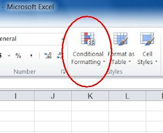
1. Click the Conditional Formatting in the ribbon of the Home TAB.

Pull down menu will open.

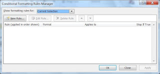
2. Click Manage Rules...
This window will open

3. In the above window, click the New Rule… button
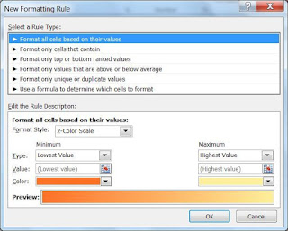
This window will open
 

4. Click the second line
   „Format only cells that contain
This window will open

5. Click the down arrow at 'Cell Value' and select the line 'Errors'
  

The window will look like this:

 

6. Click the Format… button

The next window will open




7. Click the down arrow of the 'Automatic' field

Colors pallet will open.
Select No-Color (or white color) for text and click the OK button.

The next window will show up.

8. Click the cursor in the beginning of the field Applies to

Press the keyboard Del key to delete all the text in the Applies to field.

With the mouse, mark the area in which the #N/A error will be hidden, let's say cells C3 through C10 in the above example and press the keyboard's Enter key.

If this step was done correctly the text in the Applies to field will show

=$C$3:$C$10

Click the OK button to complete the process.

Now cells with #N/A, like C4 and C8, will look empty.

C) Hide #N/A result in Excel's print out

1. Open the Page Setup, in the Page Layout TAB

2. Click the Sheet TAB, click the pulldown arrow, select <blank>, OK

 * * *

Replacing #N/A result with zero or with text message, in Excel

Displaying a neat result table without the #N/A text inserted automatically by the Excel can be done by using the IF function with the ISNA function.

The syntax of the ISNA function is:
=ISNA(cell location)

If the content of the cell at ‘cell location’ is #N/A the function returns TRUE otherwise FALSE. The idea is to use IF function to replace the content of the cell based on the TRUE/FALSE result received from the ISNA function.

Simple Examples
Let’s say that cell F5 contains the following formula:
=IF(ISNA(B5),0,B5)
In this example if cell B5 is #N/A then the IF function will display in cell F5 the number 0 (zero).
When B5 is not #N/A, the value in cell F5 will be the same as B5. It could be a number or a letter or text.

=IF(ISNA(B5),"Entry is out of range","Entry is OK")
The above formula was written in cell F5.
In this example when cell B5 is #N/A then cell F5 will display the message “Entry is out of range". When B5 is not #N/A then F5 will display the message “Entry is OK”.

Advance Example
There are two tables and cell F5 for message display, as in the below picture.

The content of cell A5 is entered by the user and should be one letter between A to D.

The value of cell B5 in Table-1 is taken from column B of Table-2 with LOOKUP function depends on the entry of user's input in cell A5. The content of B5 is:
=VLOOKUP(A5,A9:B12,2,0)

Cell C5 contains the number 1.

Cell D5 sums the value of B5 and C5.
=B5+C5

Cell F5 displays text message that gives feedback about the data that was entered in A5, if the data is A to D, then F5 will display “Entry is OK”, for any other input F5 will display “Entry is out of range”

Table-1 and Table-2 can be placed on different sheets or workbook.

When someone enters the letter E in cell A5 then Table-1 will look like this:

Cells B5 and D5 will show #N/A. Since the input data E can’t be found in Table-2, the VLOOKUP function in cell B5 will return #N/A and the formula in D5 will not be able to do the sum of B5+C5 thus will also return #N/A.

Let’s say that column B in Table-2 can contains only positive numbers except zero (0). We can replace now the #N/A in cell B5 with 0. This will enable Excel to do the sum in D5 and this will indicate to F5 that the input data was out of range.

To replace #N/A in B5 with zero, we will change the content of B5 to the following:
=IF(ISNA(VLOOKUP(A5,A9:B12,2,0)),0,(VLOOKUP(A5,A9:B12,2,0)))

After this change when the input data in A5 will cause #N/A in B5, the above IF function will replace it to 0.

As can be seen in the above picture, replacing the #N/A of cell B5 with zero (0) enabled Excel to do the sum in D5 though cell D5 shows now 1 which is the sum of 0 (B5) + 1 (C5).

Pay attention that the input data E is out of range but F5 message says “Entry is OK” since cell F5 checks cell B5 for not having #N/A but now B5 has the number zero so the check pass to display the positive message “Entry is OK”.

In order to correct the message displayed in F5 we will add IF function in the existing IF function and the content of cell F5 will be:
=IF(ISNA(B5),"Entry is out of range",IF(B5=0,"Entry is out of range","Entry is OK"))
The message in F5 will show now the correct message as in the below picture:

* * *

Copy worksheet from file to file without the links, in Excel 2010

After copying a sheet from Excel File1 to Excel File2, all the functions on the copied sheet in File2, will be linked to File1.

For example, there are two Excel files. Each file includes two sheets. In each file the names of the two sheets are identical. One sheet named Sheet-A the other sheet named Summary.

After copying the Summary sheet from File1 to File2, the content of a cell, in the sheet Summary that has been just copied to File2, will look like this:

=VLOOKUP(A10,'[FILE1.xls]Sheet-A'!$D$2:$K$100,5,0)

As can be seen the data in Summary sheet of File2 is taken now from Sheet-A of File1 while we want it to be taken from Sheet-A of File2.

If the links to File1 will be removed the data in the Summary sheet of File2 will be taken from Sheet-A of File2 its self and not from File1.

After removing the links, the content of a cell in File2 will look like this:
=VLOOKUP(A10,'Sheet-A'!$D$2:$K$100,5,0)

Now the VLOOKUP function takes the data from Sheet-A of File2.

Option 1

Remove the text [FILE1.xls] from all formulas in the sheet Summary of File2 by the Find and Replace feature exist in Excel.

Option 2
Remove all the links from the sheet Summary of File2 through the Edit Links window:

1. Click the square at the top let corner of the sheet, left to column A, to select the entire Sheet.

                                                

2. Click the Data TAB

3. Click the Edit Links button

4. Click the Change Source button

        Pop up window will open to explore file locations

5. Go to the location of File2.xls and click the Open button

Clicking the Open button after File2.xls is displayed in the ‘File name:’ field.
The above window will automatically close and the next window will show up.

        The line with the link to File1.xls has been removed automatically.

6. Click the Close button to complete the process

Done, now all functions in File2 take the data from Sheet-A of File2.

* * *